Measured electron beam parameters and their standard deviation as well as radiator and collimator properties
are the basic input for calculations based on the Monte Carlo technique.
Starting from a given number of electrons Ne, depending on the desired statistical accuracy,
a certain set of physical values are chosen randomly in parameter space.
First the direction of an incident electron
![]() with energy E0 impinging at
with energy E0 impinging at
![]() on the radiator
is chosen from the beam energy
on the radiator
is chosen from the beam energy
![]() and divergence
and divergence
![]() distributions, which are assumed
to be of Gaussian shape with known parameters
distributions, which are assumed
to be of Gaussian shape with known parameters
![]() ,
,
![]() and
and
![]() respectively.
The mean polar angle deviation
respectively.
The mean polar angle deviation
![]() from the incident direction depend via
Molières theory[11] on the depth z of the bremsstrahl process in the radiator,
which is chosen randomly from a homogenous distribution within the radiator thickness zR.
To calculate the coherent bremsstrahlung for this particular electron the lattice has to be
rotated into its coordinate system, involving a transformation of the crystal angles
from the incident direction depend via
Molières theory[11] on the depth z of the bremsstrahl process in the radiator,
which is chosen randomly from a homogenous distribution within the radiator thickness zR.
To calculate the coherent bremsstrahlung for this particular electron the lattice has to be
rotated into its coordinate system, involving a transformation of the crystal angles ![]() .
The total transversal electron deflection
.
The total transversal electron deflection
![]() due to multiple scattering and beam divergence
and the transformation of the crystal
due to multiple scattering and beam divergence
and the transformation of the crystal
![]() axis in the electron system
axis in the electron system
![]() is calculated (eq. A5c and fig. 2).
Then a lattice vector is chosen uniformly in reciprocal space
is calculated (eq. A5c and fig. 2).
Then a lattice vector is chosen uniformly in reciprocal space
![]() with the Miller indices h,k,l,
the intensity
with the Miller indices h,k,l,
the intensity
![]() is calculated with these parameters
is calculated with these parameters
![]() and the photon momentum
and the photon momentum
![]() is transformed back in the lab system.
The resulting cross section is differential in photon energy k and angle, which is
the azimuthal (
is transformed back in the lab system.
The resulting cross section is differential in photon energy k and angle, which is
the azimuthal (![]() )
in coherent bremsstrahlung and is the polar angle (
)
in coherent bremsstrahlung and is the polar angle (
![]() )
in the incoherent case.
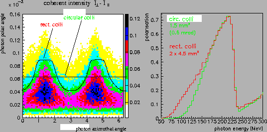
As an example the polarisation for a rectangular collimator compared to a circular one,
both producing the same tagging efficiency, is shown in fig. 3.
)
in the incoherent case.
As an example the polarisation for a rectangular collimator compared to a circular one,
both producing the same tagging efficiency, is shown in fig. 3.
 |